How To Add Conditional Sum In Excel
Steps for Adding Task Names to the Right Side of Gantt Bars in Excel. On the Home tab click Conditional Formatting in the Styles group.

How To Calculate Conditional Sum Of A Range Of Cells Using Single Criterion In Excel 2016 Youtube
TableSelectRows Grouped Rows each Account 1001 Account1001 Sum.
How to add conditional sum in excel. Udemy and the range that we would like to be calculated if match is found is Net Sales. You need to copy the below UDF put it in a module in your workbook. At this point you could choose Custom Format from the With controls dropdown.
2 Select the column name that you will sum and then click the Calculate Sum. You are using a incorrect UDF to sum cells based on conditional formatting. You use SUMIFS in Excel to find a conditional sum of values based on multiple criteria.
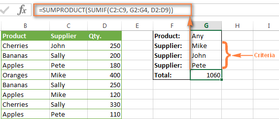
This is an example of concatenation. Array constant using OR logic forces SUMIFS function to sum numbers based on either of the multiple criteria in an array result and finally SUMfunction add up those array results like. Compared to SUMIF the SUMIFS syntax is a little bit more complex.
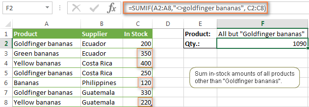
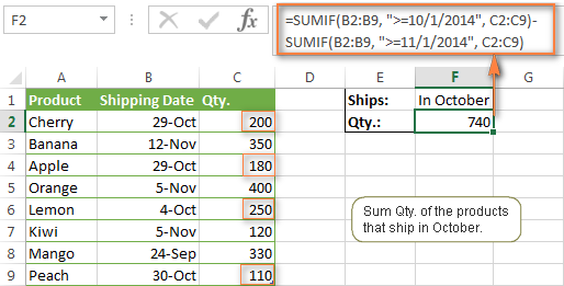
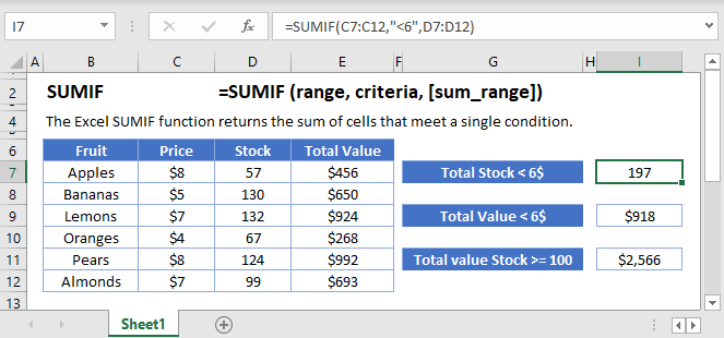
The condition that you want to check. Sum the values based on another column if only is certain text. Sum the values in cells B2B10 if a corresponding value in column A is less than 10.
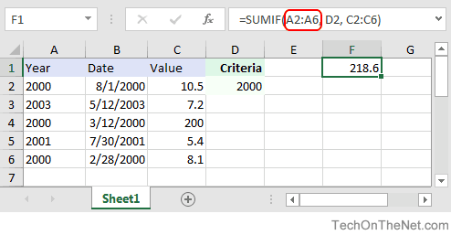
Select the data range A2A7. Now go to the cell where we need to see the output and type the sign Equal. SUMIFrange A1 Where A1 is a reference to a cell that contains the threshold number.
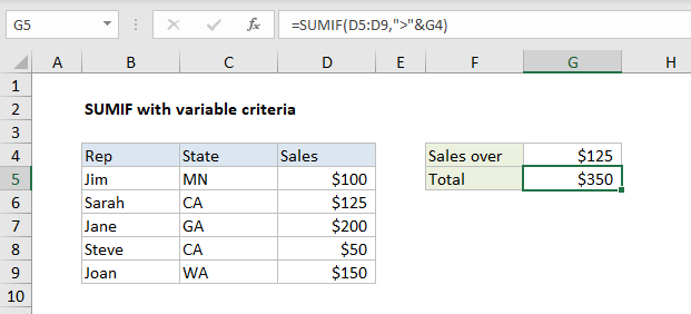
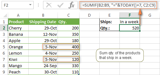
As we can see below column C has numbers with some background color. If you want to put the threshold amount on the worksheet so that it can be easily changed use this formula. SUMIFrangecriteriasum range This function would allow us to calculate the sum of range specified based on our condition applied to the criteria range.
If you just want to sum the values in column B which corresponding cell content only is KTE of column A please use this formula. SUMSUMIFSsum_range criteria_range criteria1criteria2criteria3 SUMvalue1 value2. Then use it in your workbook SumConditionColorCellsCellsRange As Range ColorRng As Range like this SumConditionColorCellsO9O40N6.
I cannot fill your template for you. 1 Select the column name that you will sum based on and then click the Primary Key button. For example the IF function uses the following arguments.
IFERRORREPTxB4B12-F1 It will repeat the character x based on the task duration from the projects start date. Sum if equal to can be omitted SUMIFA2A10 D1 or SUMIFA2A10D1 Sum the values in cells A2A10 that are equal to the value in cell D1. 3 Click the Ok button.
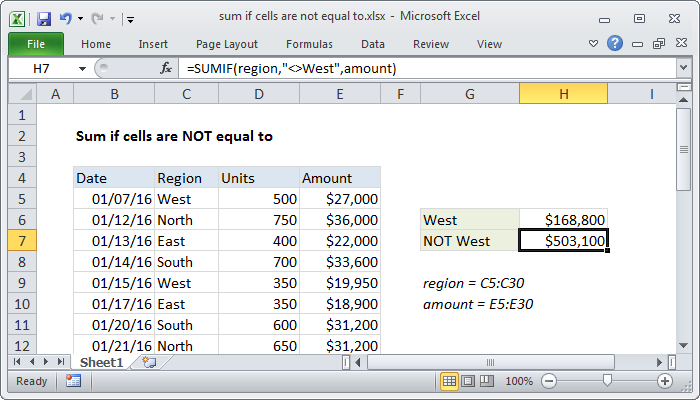
In the example shown cell G6 contains this formula. In the opening Combine Rows Based on Column dialog box you need to. The value to return if the condition is False.
SUMIFS D2D11 In other words you want the formula to sum numbers in that column if they meet the conditions. Sum if not equal to SUMIFA2A10 D1 B2B10. In our example our criteria range is Web Platform.
Choose Highlight Cells Rules and then choose Greater Than. Very Easy way to add up in Excel based on a certain conditionIf your task requires adding only those cells that meet a certain condition or a few conditions. I looked at your file.
Now lets go to the steps to add floating task names next to the bars. Now as we need to sum the numbers so from the drop-down of SUBTOTAL Function select 9 which is for sum. And search and select the SUBTOTAL function as shown below.
In the formula for the new column I simply replaced the parameter I used for the filter with a dynamic reference to the Account column combining it with the next step drill down. C6C22 our condition is the web platform used. In the resulting dialog enter 4.
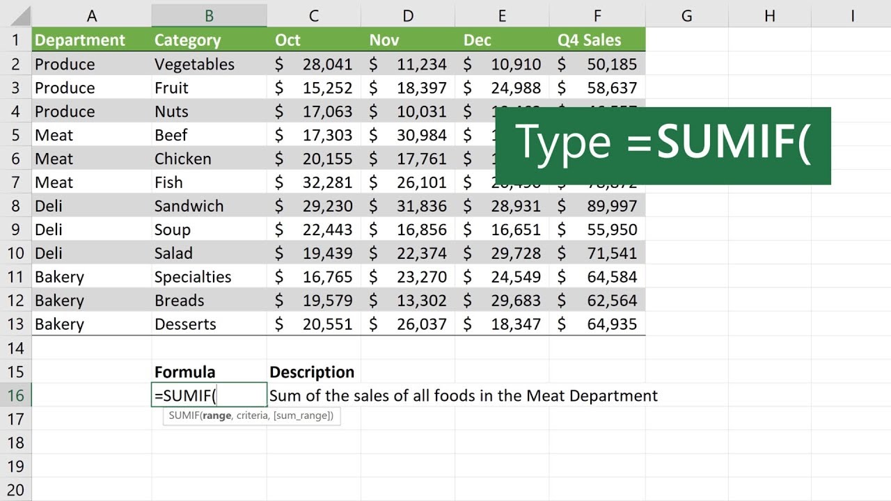
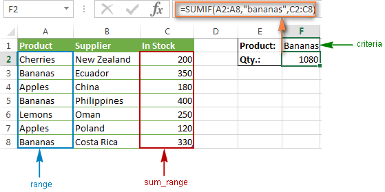
The first step is to specify the location of the numbers. The value to return if the condition is True. SUMIF A2A6KTEB2B6 A2A6 is the data range which you add the values based on KTE stands for the criterion you need and B2B6 is the range you want to sum and then only the text is KTE in column A which relative number in column B will add.
You can use the AND OR NOT and IF functions to create conditional formulas. In cell F4 insert the following formula. To sum if cells contain specific text you can use the SUMIF function with a wildcard.
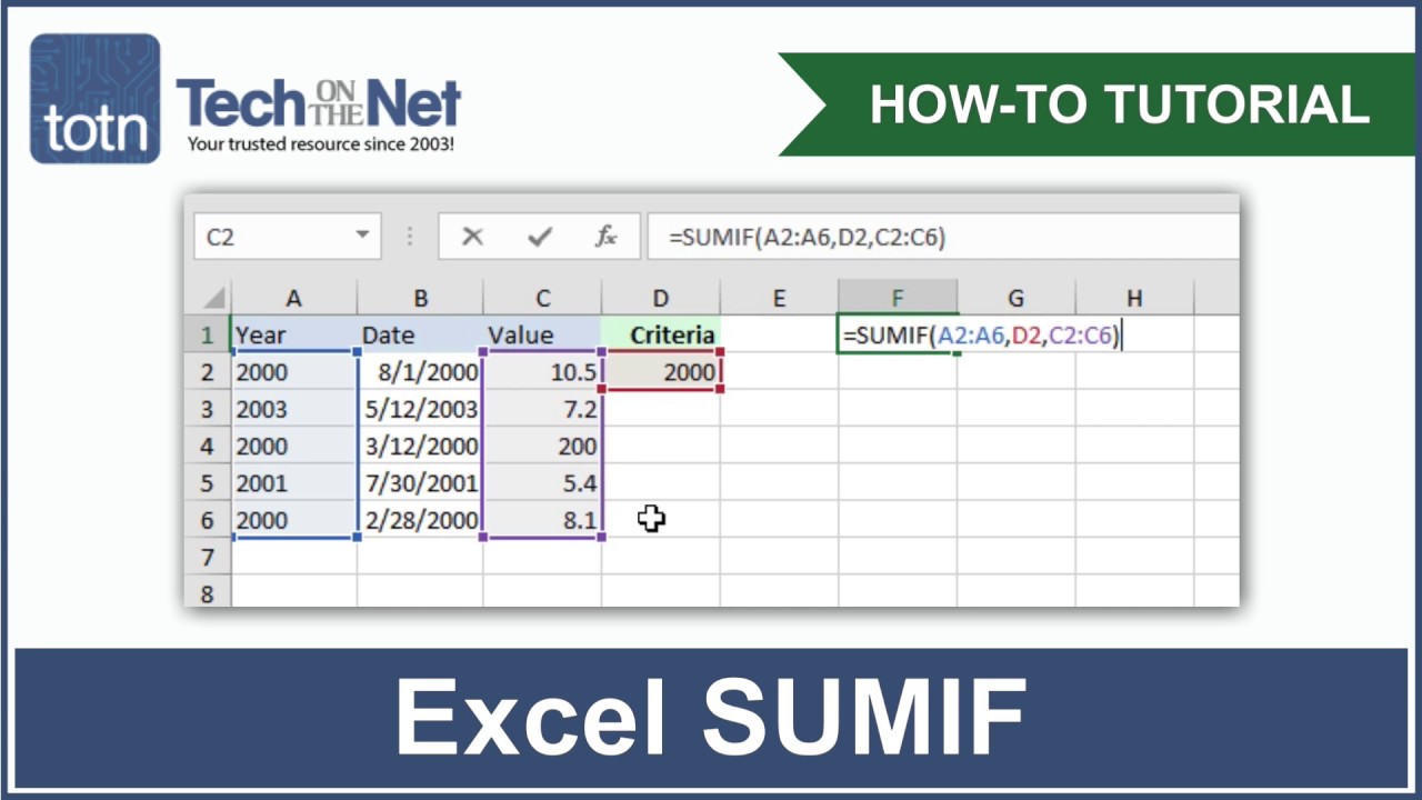
The SUMIFS function was introduced in Excel 2007 so you can use it in all modern versions of Excel 2019 2016 2013 2010 and 2007. That cell range is the first argument in this formulathe first piece of data that the function requires as input. Learn how to calculate conditional sum of a range of cells using single criterion in Excel 2016 - Office 365.
SUMIF C5C11t-shirt D5D11 This formula sums the amounts in column D when a value in column C contains.
How To Use Sumif Function In Excel To Conditionally Sum Cells
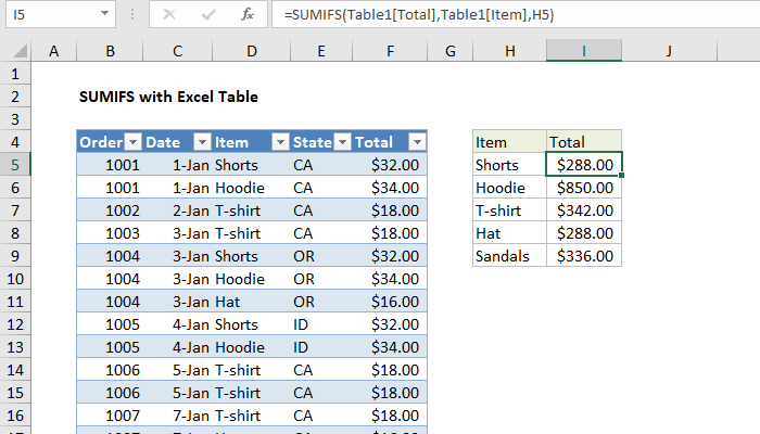
Excel Formula Sumifs With Excel Table Exceljet
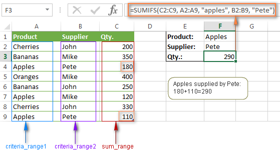
Excel Sumifs And Sumif With Multiple Criteria Formula Examples
How To Use The Sumif Function In Microsoft Excel Youtube
Excel Formula Sum If Cells Are Not Equal To Exceljet

Sumif And Countif In Excel
How To Use Sumif Function In Excel To Conditionally Sum Cells

How To Use The Sumif Function In Excel Step By Step
Ms Excel How To Use The Sumif Function Ws
How To Use The Excel Sumif Function Exceljet
How To Use Sumif Function In Excel To Conditionally Sum Cells
Excel Sumifs And Sumif With Multiple Criteria Formula Examples

How To Use The Excel Sumifs Function Exceljet
How To Use The Sumif Function In Excel Youtube

What To Do If Excel Sumif Is Not Working

How To Use The Excel Sumif Function Exceljet
How To Use Sumif Function In Excel To Conditionally Sum Cells
Sumif Sumifs Functions Sum Values If Excel Google Sheets Automate Excel

Excel Tips How To Use Sumif Function In Excel With Pictures